
-
Layer with depth-dependent properties over homogeneous halfspace
- Tested algorithms:
This benchmark case was applied to the following programs: SOFI2D (transformed), SOFI3D, SPECFEM and Gemini
- Scale:
Shallow seismic data
Benchmark case: Layer with depth-dependent properties over homogeneous halfspace
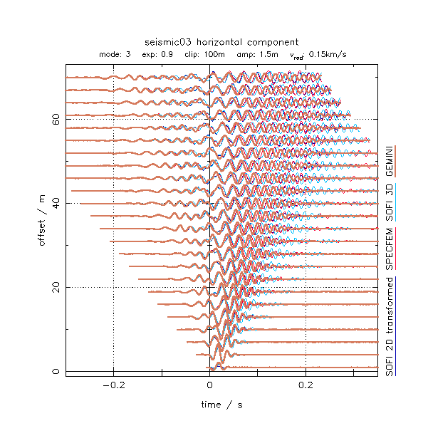
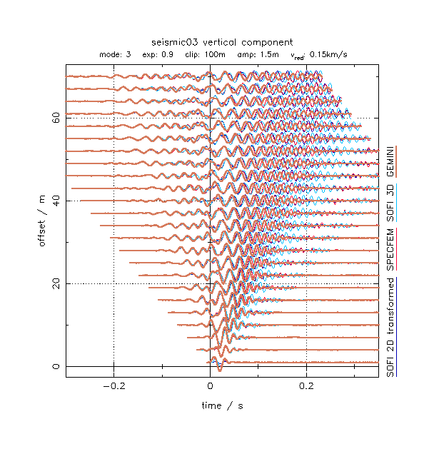
Model description
The benchmark model for this case was derived from a field data set (see http://www.opentoast.de/Bietigheim.php for further information about the data set and the derived subsurface model). Although the subsurface model was derived from field data, this benchmark calculation is not a simulation of recorded data. Purely elastic wave propagation is used for the benchmark test, while field data is significantly attenuated by anelasticity.
The model consists of a layer over homogeneous halfspace, where the material parameters continuously vary with depth within the layer. This type of depth-dependence is typical for unconsolidated near-surface sediments overlying a hard-rock. A vertical force source is used as source. Download the model description for a detailed description of the benchmark test including the definition of the material parameters and the characteristics of the source and the acquisition geometry.
Compared algorithms
In this benchmark test four different forward solvers are compared: SPECFEM3D, Gemini II, SOFI3D and SOFI2D where results of SOFI2D are transformed to equivalent point-source seismograms. A description of the transformation is provided for download. Please note that proper physical amplitudes of the source are only implemented in SPECFEM3D and SOFI2D.
Time series for download
The calculated time series are provided for download.
The plots displayed on the left and additional zoomed views are provided for download (PDF file). The seismogram displays are produced with refractx. Plot parameters are given in the subtitle of each plot.
The parameter settings used for the plots are given in the label of each plot.
- mode: scaling mode
- 1: scale traces individually
- 2: scale all traces to first trace as reference
- 3: scale all traces to a common offset trace of each dataset as reference
- exp: traces are scaled by offset-dependent factor of (r/1m)exp where r is the offset
- clip: clipping level
- amp: amplitude level
- vred: timescale is reduced by tred=t-r/vred